The 3.5mm Connector Is a Transmission Line

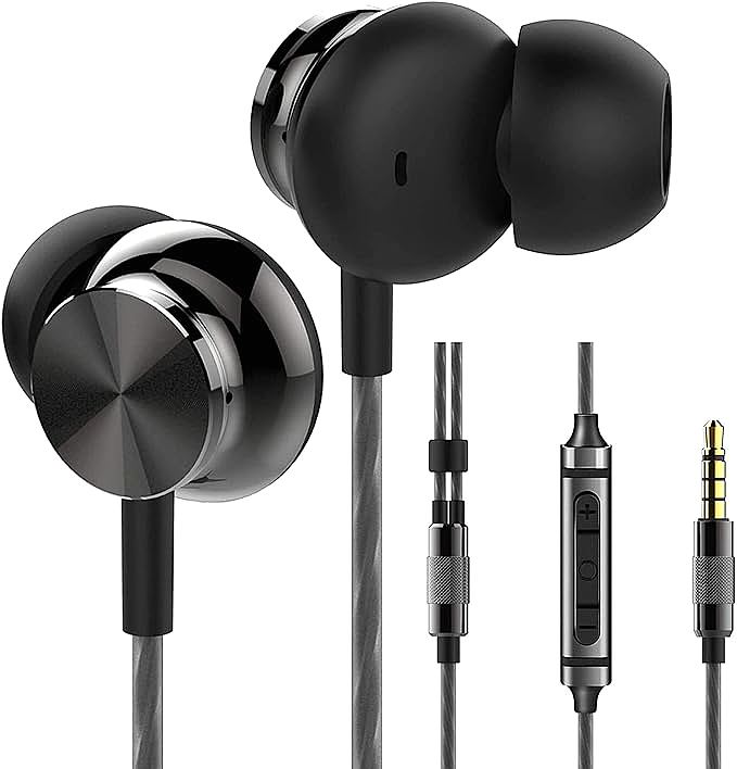
Betron BS10 Wired Headphones
You plug a pair of wired headphones — say, the Betron BS10 — into a laptop, press play, and sound comes out. Simple enough. But somewhere between the digital-to-analog converter and the tiny speaker in your ear, the audio signal passes through a small cylindrical connector that most people treat as a piece of wire. It is not. That 3.5mm jack and the cable attached to it behave as a transmission line, with measurable distributed capacitance, characteristic impedance, and frequency-dependent losses that shape the signal before it ever reaches your ears.
This is not audiophile mysticism. These are electrical engineering fundamentals, measurable with a multimeter. Understanding how a headphone cable actually works removes guesswork from diagnosing audio problems and from choosing equipment for latency-sensitive uses like gaming or live monitoring.
A 3.5mm Cable Is Not a Wire
A piece of wire has resistance. A transmission line has resistance, inductance, capacitance, and conductance, all distributed along its length. The distinction matters when the physical length of the cable becomes a meaningful fraction of the signal wavelength. For audio frequencies (20 Hz to 20 kHz), wavelengths range from 15,000 kilometers down to 15 kilometers. A 1.2-meter headphone cable is electrically short at these frequencies, so it will not exhibit the standing-wave resonance behavior seen in RF or high-speed digital transmission lines.
But that does not mean the distributed parameters are irrelevant. A typical headphone cable carries two conductors (signal and ground for each channel), and the geometry between those conductors creates parasitic capacitance. Along with the series inductance of the wire, this capacitance forms a passive network that interacts with whatever load is connected at the end.
The characteristic impedance of a transmission line is given by:
Z_0 = sqrt(L / C)
where L is the inductance per unit length (henries per meter) and C is the capacitance per unit length (farads per meter). For a typical headphone cable, L is approximately 0.5 microhenries per meter and C is approximately 100 picofarads per meter. Substituting:
Z_0 = sqrt(0.5 x 10^-6 / 100 x 10^-12) = sqrt(5000) ~ 70.7 ohm
This value is the impedance a signal "sees" as it propagates along the cable. It is not the same as the DC resistance of the wire, which is typically under 1 ohm per meter for copper conductors. The characteristic impedance governs how the signal interacts with impedance discontinuities at the connector and at the load.
A 3.5mm TRS (Tip-Ring-Sleeve) connector has three contacts that create a transition region between the cable and the headphone driver. The impedance mismatch between the cable (~70 ohm) and a typical 16 ohm earphone load means that some portion of the signal energy reflects at the junction. At audio frequencies, this reflection is negligible in magnitude, but the mismatch interaction with distributed capacitance does produce measurable effects on high-frequency response.
The TRS plug carries audio only. Headset cables add a fourth conductor (TRRS), and that extra ring carries the microphone signal down the same physical cable, sharing its ground with both audio channels. Call quality therefore depends on the connector as much as the drivers: every contact resistance and oxide layer sits in series with a microphone signal that is an order of magnitude smaller than line-level audio, so a marginal contact that would never bother a music signal can dominate a call.
Distributed Capacitance Forms a Low-Pass Filter
The most significant cable-related effect on audio frequency response is not resistance or inductance alone. It is the combination of the cable's distributed capacitance with the output impedance of the source device. Together, they form a first-order low-pass filter.
The Formula: fc = 1 / (2pi C Zout)
The -3 dB cutoff frequency of this filter is:
fc = 1 / (2pi C Zout)
where C is the total cable capacitance (farads) and Zout is the output impedance of the source (ohms). This formula tells you the frequency above which the signal begins to attenuate at a rate of 6 dB per octave.
Total cable capacitance scales linearly with length:
C_total = C_spec x length
For a cable with a specific capacitance of 100 pF per meter and a length of 1.2 meters, C_total = 120 pF. For a 3-meter cable, C_total = 300 pF. A lower-quality cable with tighter conductor spacing might have C_spec as high as 300 pF/m, giving 900 pF over 3 meters.
Real-World Examples: Different Cables on Different Sources
The cutoff frequency depends heavily on the source output impedance, not just the cable. Here are three scenarios:
Scenario A and B: a 1-meter cable (100 pF) on a smartphone with Zout = 3 ohm gives fc ~ 530 MHz, and a 3-meter cable (300 pF) on a portable DAC with Zout = 10 ohm gives ~ 53 MHz. Both are far above the audible range; with modern low-impedance sources the cable has no measurable effect.
Scenario C: 3-meter low-quality cable (900 pF) connected to a vacuum tube amplifier with Zout = 10,000 ohm (10 kohm).
fc = 1 / (2pi x 900 x 10^-12 x 10,000) ~ 17.7 kHz
This sits at the upper bound of human hearing, and a trained listener on high-quality material might perceive a slight reduction in "air" or brilliance.
The table below summarizes these calculations:
| Cable Length | Cable Capacitance | Source Zout | Cutoff Frequency | Audible Effect? |
|---|---|---|---|---|
| 1 m | 100 pF | 3 ohm | ~530 MHz | No |
| 3 m | 300 pF | 10 ohm | ~53 MHz | No |
| 3 m | 900 pF | 10 kohm | ~17.7 kHz | Yes |
The takeaway is direct: the cable alone is almost never the limiting factor with modern low-impedance sources. The problem emerges when a high-impedance source is paired with a long, high-capacitance cable.
How Cable Length and Physical Stress Change Capacitance
Capacitance between two parallel conductors depends on their geometry. The governing relationship for a coaxial arrangement is:
C = (2pi eps_0 epsr L) / ln(b/a)
where eps_0 is the permittivity of free space (8.854 x 10^-12 F/m), epsr is the relative permittivity of the dielectric insulation between conductors, L is the cable length, b is the outer conductor radius, and a is the inner conductor radius.
For a headphone cable, the geometry is more complex than a simple coaxial structure (multiple conductors twisted or bundled), but the principle holds: closer conductor spacing means higher capacitance per meter. This is why flat cables and ribbon-style cables often have higher capacitance than round cables with the same wire gauge.
Repeated bending or kinking near the connector deforms the dielectric spacing locally, creating a capacitance hotspot. Manufacturers specify a minimum bending radius, often 4 to 8 times the outer diameter; below it, the dielectric deforms and conductor spacing shrinks. A severe kink can raise local capacitance 20-50% over the straight section, lowering the cutoff frequency through that segment.
Dielectric material also matters: polyethylene sits near a dielectric constant of 2.3, while PVC, the most common consumer insulation, ranges from 3.0 to 4.5 depending on plasticizer content. Higher constants mean higher capacitance per meter; rigid PVC at epsr = 4.5 roughly doubles the per-meter capacitance of foamed polyethylene at epsr = 1.5. Manufacturers rarely publish these figures, making direct comparison difficult without measurement.
Output Impedance Shifts the Cutoff Frequency
The formula fc = 1 / (2pi C Zout) reveals something that cable discussions almost always miss: the source device matters as much as the cable. Output impedance (Zout) is the internal resistance that the amplifier or DAC presents to the load.
A modern smartphone headphone jack typically has Zout between 1 and 5 ohm. A dedicated headphone amplifier might be 0.1 ohm or lower. But vintage equipment and some consumer electronics can have much higher output impedance: 100 ohm, 600 ohm, or even 10 kohm for some vacuum tube designs.
The relationship is inverse: higher Zout lowers the cutoff frequency, so the cable's capacitance starts affecting audio response at a lower frequency. Here is how the same 2-meter cable (200 pF) behaves with different sources:
| Source Type | Typical Zout | fc with 200 pF cable |
|---|---|---|
| Modern smartphone | 3 ohm | ~265 MHz |
| Desktop headphone amp | 0.5 ohm | ~1.6 GHz |
| Pro audio interface | 50 ohm | ~16 MHz |
| Vintage receiver | 600 ohm | ~1.3 MHz |
| Tube amplifier | 10 kohm | ~80 kHz |
Real-world cables, especially ones that have been bent, aged, or exposed to moisture, often exceed the 100 pF/m specification, and the degraded-cable case above shows how quickly that margin disappears on a high-impedance source.
This is the mechanism behind the commonly reported phenomenon of "cable differences" being audible on tube amplifiers but inaudible on solid-state equipment. The difference is not the cable itself changing. The source impedance determines whether the cable's inherent capacitance becomes a frequency-limiting factor.
Guitar players have known this for decades and call it "tone suck": a 10 kohm effects loop driving 5 meters of 300 pF/m cable pushes the cutoff near 10 kHz, and the air in a cymbal crash rolls off with it.
Gold Plating Prevents Contact Resistance Drift
Oxidation of audio connectors is a slow, invisible process that increases contact resistance over months and years. The mechanism is electrochemical: when two dissimilar metals are in contact in the presence of moisture and oxygen, galvanic corrosion occurs. The rate depends on the difference in standard electrode potentials.
Gold has a standard electrode potential of +1.69 V. Copper is +0.34 V. Nickel, commonly used as a cheaper connector plating, is -0.26 V. The larger the potential difference between the connector plating and the contacts it touches, the faster corrosion proceeds.
A bare copper connector exposed to humid air forms a thin layer of copper oxide (CuO) within weeks. This oxide layer is a semiconductor with much higher resistivity than metallic copper. For a connector carrying millivolt-level audio signals, even a few hundred ohms of additional contact resistance at the oxide layer creates a measurable voltage divider that attenuates the signal.
Gold plating works because gold is a noble metal: it does not form an oxide layer under normal atmospheric conditions. A gold-plated connector maintains a stable, low contact resistance indefinitely, provided the gold layer is thick enough to be pinhole-free (typically 0.5 to 1.0 micrometers for audio connectors).
Nickel plating offers moderate protection. Nickel oxide forms more slowly than copper oxide and has lower resistivity, but it still degrades over time, especially in humid environments. The typical lifespan comparison:
- Bare copper connector: measurable oxidation within weeks, significant contact resistance increase within 6-12 months
- Nickel-plated connector: stable for 2-5 years under normal indoor conditions
- Gold-plated connector: stable for decades under normal conditions
For headphones that are plugged in once and left connected, oxidation is rarely a problem. For equipment that is frequently connected and disconnected, or stored in humid environments, gold plating provides a measurable reduction in long-term maintenance.
What a Capacitance Reading Reveals
Measuring a cable's capacitance requires only basic test equipment and confirms whether a cable is performing within specification. Two methods are practical for home use.
Method 1: LCR Meter
An LCR meter measures inductance (L), capacitance (C), and resistance (R) directly. Set the meter to capacitance mode, connect the probes to signal and ground at one end of the cable, and leave the far end open. The reading is total capacitance; divide by length in meters for pF/m.
Method 2: RC Time Constant
If no LCR meter is available, a known resistor and an oscilloscope can determine capacitance. Connect a known resistance R in series with the cable and apply a step voltage. Measure the time it takes for the voltage across the cable to reach 63.2% of the applied voltage (one time constant, tau). Then:
C = tau / R
For example, with R = 10 kohm and a measured tau = 1.2 microseconds, C = 1.2 x 10^-6 / 10,000 = 120 pF.
Typical values for common cable types:
| Cable Type | Specific Capacitance (pF/m) |
|---|---|
| Standard headphone cable | 80 - 150 |
| Coaxial audio cable (RG-59) | 60 - 70 |
| Cheap thin cable (high-density) | 200 - 350 |
| Specialty low-capacitance cable | 40 - 60 |
A cable measuring above 200 pF/m is likely degraded or poorly constructed. If you suspect a cable of causing high-frequency loss, measuring its capacitance provides a concrete number to compare against specifications. Always measure with the cable uncoiled and laid straight. Coiling introduces stray capacitance between adjacent loops that inflates the reading above the cable's true per-meter specification.
Wired Versus Wireless: When Latency Matters

The transmission line discussion above covers frequency response. But for many users, the more pressing question is delay. Audio latency is the time between a signal being generated and reaching the listener's ear. In gaming, live music monitoring, and professional audio production, latency determines whether the experience feels natural or disconnected.
Wired 3.5mm analog connections have near-zero latency: the electrical signal propagates through the cable at a significant fraction of the speed of light. For a 1.2-meter cable, the propagation delay is approximately 4 to 6 nanoseconds. Add the DAC conversion time, and the total system latency for a wired connection is typically 0 to 5 milliseconds.
Wireless connections add protocol overhead, compression, transmission, and decompression steps. The table below shows measured latency ranges for common connection types:
| Connection Type | Typical Latency |
|---|---|
| Wired 3.5mm analog | 0 - 5 ms |
| USB digital audio | 5 - 15 ms |
| 2.4 GHz wireless dongle | 10 - 30 ms |
| Bluetooth aptX Low Latency | 30 - 60 ms |
| Bluetooth SBC / AAC | 100 - 200 ms |
Audio-visual synchronization degrades noticeably above roughly 45 milliseconds. For competitive gaming where audio cues (footsteps, gunshots) must align with on-screen action, a wired connection eliminates an entire category of timing error. For casual music listening, the latency of modern Bluetooth codecs like aptX Low Latency is below the perception threshold for most listeners, though codec choice changes how wireless audio sounds beyond timing alone.
The difference between 5 ms and 150 ms is not subtle in a rhythm game or a first-person shooter. It is the difference between reacting to a sound and hearing it after you have already moved, part of why signal path engineering still matters for wired earbuds. This is one reason professional stage musicians and audio engineers continue to rely on wired monitoring systems despite the convenience of wireless.
The Skin Effect at Audio Frequencies
One additional physical phenomenon worth addressing: the skin effect. At high frequencies, current tends to flow only near the surface of a conductor rather than through its full cross-section. The skin depth is:
delta = 1 / sqrt(pi f mu sigma)
where f is frequency, mu is permeability, and sigma is conductivity. For copper at 20 kHz (the upper limit of human hearing):
delta = 1 / sqrt(pi x 20,000 x 4pi x 10^-7 x 5.8 x 10^7) ~ 0.46 mm
A typical headphone wire has a radius of 0.1 to 0.2 mm, well below that skin depth, so the full cross-section carries current evenly across the audio band. Skin effect in headphone cables is not a factor in audio quality.
This is a case where the physics directly contradicts marketing claims about "oxygen-free copper" or "silver-plated" conductors providing audible benefits at audio frequencies.
When Connectors Fail: Reading the Symptoms
When one channel drops out or crackles when the connector is moved, the root cause is almost always mechanical: a worn contact, oxidized plating, or a fractured solder joint inside the plug. A systematic approach narrows the fault quickly.
The Plug-and-Rotate Test
Insert the connector fully, then slowly rotate it 360 degrees while audio plays. If the audio cuts in and out during rotation, the contact between the plug and jack is intermittent. This points to worn or oxidized contacts in either the plug or the jack.
The Wiggle Test
Hold the connector steady and gently flex the cable near the plug. If audio cuts out, the fault is likely a broken conductor inside the plug, where the cable meets the strain relief. This is the most common failure mode for headphones that are frequently pocketed or wrapped.
The Substitution Test
Test the headphones on a different device, and test a different set of headphones on the original device. This isolates whether the fault is in the headphones or the jack.
If the fault follows the headphones, cleaning the plug with a contact cleaner and gently re-bending the jack's internal contacts (using a thin pick) often restores connection. If the fault is in the jack, the jack itself may need replacement or professional cleaning.
The physics is straightforward: contact resistance at the plug-jack interface must stay low and stable, because any oxide or misalignment that raises it forms a voltage divider that eats into a millivolt-level signal.
The 3.5mm connector may look like a piece of stamped metal, but it completes a transmission line, presents a defined characteristic impedance, and carries a signal that arrives faster than any wireless protocol yet devised. Understanding the physics of what happens inside that cable does not require an engineering degree. It requires only the willingness to treat a piece of wire as what it actually is: an electrical system with measurable, predictable, and sometimes audible behavior.